AI621

Initials

Since native Python does not support loading the .cr2 file extension, we will be using the rawpy and the numpy library to open and manipulate our image.
rawpy.imread and rawpy.raw_image_visible returns returns the raw values of the banana_slug.cr2 RAW image file.
We will store the values with double-precision since our operations will be conducted in the range of 0-1.


      raw_image = rawpy.imread('data/banana_slug.cr2') 

      raw_image = raw_image.raw_image_visible # values stored in uint16 

      raw_image = raw_image.astype(np.double) # convert to double

Linearization

Once we have loaded the RAW image, we will first linearize the image, indicating that we will compensate the non-linear photodiode response function near over/under-saturated regions.
Thus, we clip the values with a threshold and map the pixel values between 0-1 for further steps.


        CAMERA_MIN = 2047 

        CAMERA_MAX = 15000 

        clipped_image = np.clip(raw_image, a_min=CAMERA_MIN, a_max=CAMERA_MAX) 

        linearized_image = (clipped_image - CAMERA_MIN) / (CAMERA_MAX - CAMERA_MIN) 

         

        cv2.imwrite('1_Linearization.png', (linearized_image * 255).astype(np.uint8))

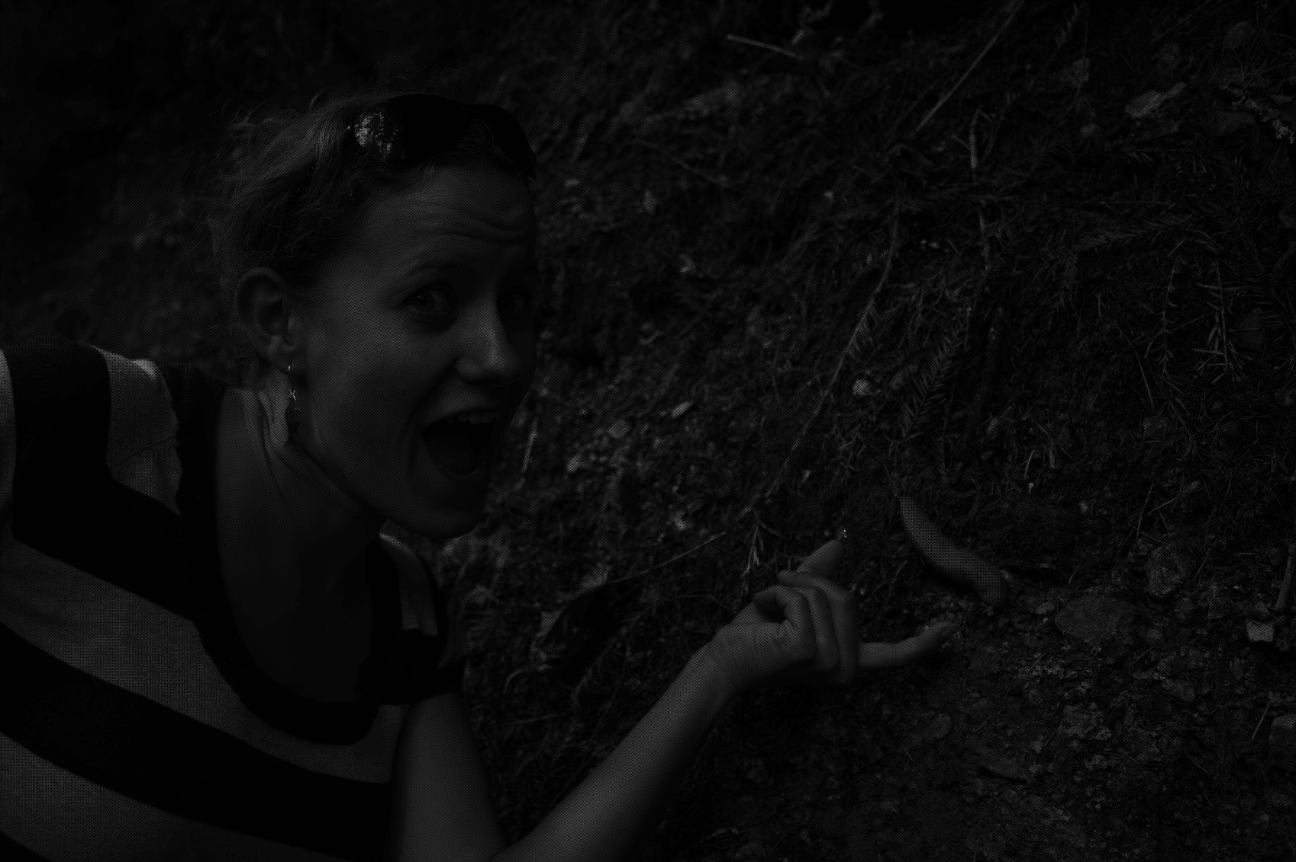
The linearized image is visualized by mapping values in the range of 0-1 to 8bit unsigned values 0-255. Notice that the image appears as grayscale since we did not assign any colors to this single channel image.

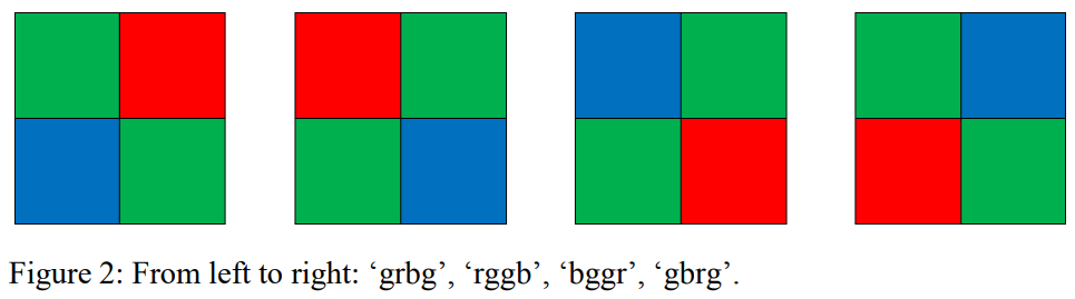
Identifying the Correct Bayer Pattern

Before assigning or adjusting the values of each pixel, we first need to the determine the Bayer pattern of the sensor. This is essential for appropriately converting a single channel image into a 3-channel RGB image. Among four possible Bayer patterns, we need to determine which pattern our camera follows.

Note that we can always search online to find already-known camera-specific configurations. Our image is taken by a Canon EOS T3 Rebel camera, which is known to have a "rggb" pattern. Let us find this out in an analytic approach by using hints from known colors. (without the help of the internet)

We infer the arrangement of the green pixels by assuming either the top-left bottom-right ("grbg" and "gbrg") or the top-right bottom-left ("rggb" and "bggr") pattern and interpolating the colors (demosaicing) for the remaining pixels.
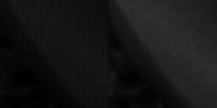
Once we perform demosaicing for the green channel, regions with high green value (e.g., yellow slug) should have high intensities all accross the slug region. However, when assuming the top-left, bottom-right pattern, we observe that pixels have alternating high, low intensities and creates checkerboard artifacts after interpolation. This is due to the fact that yellow colors have contrasting intensities of red and blue (high red and low blue). Thus, we can conclude that our camera has either the "rggb" or the "bggr" pattern.

Left - Demosaiced image assuming top-left bottom-right pattern
Right - Demosaiced image assuming top-right bottom-left pattern


        HEIGHT, WIDTH = linearized_image.shape

        

        top_right_mask = np.zeros((HEIGHT, WIDTH), dtype=np.int_)

        top_right_mask[0:-1:2, 1:-1:2] = 1

        

        bottom_left_mask = np.zeros((HEIGHT, WIDTH), dtype=np.int_)

        bottom_left_mask[1:-1:2, 0:-1:2] = 1

        

        

        top_left_mask = np.zeros((HEIGHT, WIDTH), dtype=np.int_)

        top_left_mask[0:-1:2, 0:-1:2] = 1

        

        bottom_right_mask = np.zeros((HEIGHT, WIDTH), dtype=np.int_)

        bottom_right_mask[1:-1:2, 1:-1:2] = 1

        

        # Interpolate the green channel

        green_mask_tl_br = (top_left_mask + bottom_right_mask) * linearized_image

        green_mask_tr_bl = (top_right_mask + bottom_left_mask) * linearized_image

        kernel= np.array([[0.00, 0.25, 0.00],[0.25, 0.00, 0.25],[0.00, 0.25, 0.00]])

        grayscale_tl_br = cv2.filter2D(green_mask_tl_br, ddepth=-1, kernel=kernel) + green_mask_tl_br

        grayscale_tr_bl = cv2.filter2D(green_mask_tr_bl, ddepth=-1, kernel=kernel) + green_mask_tr_bl

        

        # Show the slug region

        banana = cv2.hconcat([grayscale_tl_br[1750:1850, 3000:3100], grayscale_tr_bl[1750:1850, 3000:3100]])

        

        cv2.imwrite('2_Bayer_Pattern_Green.png', (banana*255).astype(np.uint8))

We can find the location of red and blue pixels in a similar manner by assuming the "rggb" and the "bggr" pattern and demosaicing the image accordingly. The slug region turns bright when assuming the "rggb" pattern, which means that the pixels lie in a "rggb" pattern. Leveraging already-known colors in the image helps us to identify camera parameters and configurations.

White Balance

Now that we know which pixel correspond to which color, we can perform color-related modifications. White balancing is commonly performed in the earlier stages to balance out unnecessary color cast. We can perform automatic white balancing under an assumption about the image.
The gray world assumption assumes that the average intensity of a scene is gray. Following this assumption, we scale each channel of the image so that the average red, blue, green values are the same.
Similarly, the white world assumption assumes that the maximum intensity of a scene is white. We scale each channel of the image so that the maximum red, blue, green values are a predefined white color (in this case maximum green intensity).

Left - Gray world assumption white balance
Right - White world assumption white balance

Left - Gray world assumption white balance (Demosaiced)
Right - White world assumption white balance (Demosaiced)

I choose the automatic white balanced image under the grayworld assumption since the white world assumption seems to have a redish color cast


        # RGGB

        _r = linearized_image * top_left_mask

        _g = linearized_image * green_mask

        _b = linearized_image * bottom_right_mask

        

        r_mean = np.ma.array(linearized_image, mask=1-top_left_mask).mean()

        g_mean = np.ma.array(linearized_image, mask=1-green_mask).mean()

        b_mean = np.ma.array(linearized_image, mask=1-bottom_right_mask).mean()

        

        r_max, g_max, b_max = _r.max(), _g.max(), _b.max()

        

        # might be good to prevent division-by-zero

        gray_world_wb = np.clip(_r * (g_mean / r_mean) + _g + _b * (g_mean / b_mean), 0, 1)

        white_world_wb = np.clip(_r * (g_max / r_max) + _g + _b * (g_max / b_max), 0, 1)

        

        cv2.imwrite('3_Gray_World_WB.png', (gray_world_wb * 255).astype(np.uint8))

        cv2.imwrite('3_White_World_WB.png', (white_world_wb * 255).astype(np.uint8))

        

        white_balanced_image = gray_world_wb.copy()

        # white_balanced_image = white_world_wb.copy()

Demosaicing

Our image is still a single channel image without any color related information. However, we now know the Bayer pattern of the sensor and can assign colors to each pixels. Thus we can interpolate the missing pixels to fill in the colors for all location and all RGB channels.
Specifically, we design four filters which interpolate the colors from different locations. For example, the blue pixels only cover a quarter of the whole image. Thus, the other three pixel locations must be interpolated using three different filters. In order to do so, we first mask out all other pixels besides blue. Than, we apply the diagonal, vertical, and horizonatal kernel in order to obtain the blue values for the red pixel, top-right green pixel, and bottom-left green pixel, accordingly. We sum up the results to obtain a full-resolution intensity value for all locations. The opencv-python library enabled the use of convolution filters.


        diag_kernel = np.array([[0.25, 0.00, 0.25],

                                [0.00, 0.00, 0.00],

                                [0.25, 0.00, 0.25]])

        

        cross_kernel= np.array([[0.00, 0.25, 0.00],

                                [0.25, 0.00, 0.25],

                                [0.00, 0.25, 0.00]])

        

        horizontal_kernel = np.array([[0, 0.0, 0.0],

                                      [0.5, 0.0, 0.5],

                                      [0.0, 0.0, 0.0]])

        

        vertical_kernel = np.array([[0.0, 0.5, 0.0],

                                    [0.0, 0.0, 0.0],

                                    [0.0, 0.5, 0.0]])

        

        # RGGB

        g_channel = green_mask * white_balanced_image

        interpolated_g = cv2.filter2D(g_channel, ddepth=-1, kernel=cross_kernel)

        

        g_channel = g_channel \

        + interpolated_g * (bottom_right_mask + top_left_mask)

        

        b_channel = bottom_right_mask * white_balanced_image

        interpolated_b_diag = cv2.filter2D(b_channel, ddepth=-1, kernel=diag_kernel)

        interpolated_b_horizontal = cv2.filter2D(b_channel, ddepth=-1, kernel=horizontal_kernel)

        interpolated_b_vertical = cv2.filter2D(b_channel, ddepth=-1, kernel=vertical_kernel)

        

        b_channel = b_channel \

        + interpolated_b_diag * (top_left_mask) \

        + interpolated_b_horizontal * (bottom_left_mask) \

        + interpolated_b_vertical * (top_right_mask)

        

        r_channel = top_left_mask * white_balanced_image

        interpolated_r_diag = cv2.filter2D(r_channel, ddepth=-1, kernel=diag_kernel)

        interpolated_r_horizontal = cv2.filter2D(r_channel, ddepth=-1, kernel=horizontal_kernel)

        interpolated_r_vertical = cv2.filter2D(r_channel, ddepth=-1, kernel=vertical_kernel)

        

        r_channel = r_channel \

        + interpolated_r_horizontal * top_right_mask \

        + interpolated_r_diag * bottom_right_mask \

        + interpolated_r_vertical * bottom_left_mask

        

        bgr_image = np.stack([b_channel, g_channel, r_channel], axis=-1)

        cv2.imwrite('4_Demosaicing.png', (bgr_image * 255).astype(np.uint8))

Brightness Adjustment and Gamma Correction

We can also alter the overall brightness of the image. Unlike white balancing, this will not remove or add colors to the image since it scales the values identically. I determined the scaling ratio so that the maximum grayscale value of the image will be 1.0, which was approximately 17% increase in brightness. This would prevent from pixel values to saturate.

We perform gamma correction to the image so that the image would be appropriate for display. According to the provided equation, underexposed regions are linearly scaled and most regions are gamma corrected. The image is finally clearly visible.


        # scaling

        gray_image = 0.3 * r_channel + 0.59 * g_channel + 0.11 * b_channel

        brightened_image = bgr_image * (1.0 / gray_image.max())

        cv2.imwrite('5_Brightness_Adjustment.png', (brightened_image * 255).astype(np.uint8))

        

        # gamma correction

        linear_region = brightened_image < 0.0031308

        non_linear_region = ~linear_region

        

        gamma_corrected_image = linear_region * brightened_image * 12.92 \

                + non_linear_region * ((1.055) * np.power(brightened_image, 1/2.4) - 0.055)

        

        cv2.imwrite('5_Gamma_Correction.png', (gamma_corrected_image*255).astype(np.uint8))

Compression

Finally, we save the image into a 8bit file. The original .cr2 file was 17.5 MB. The .png format is a lossless compression and compresses the image into 15.9 MB. The .jpg format is a lossy compression and we can determine the quality-compression rate trade-off. Images compressed with 95, 90, 80, and 70 JPEG quality has a size of 2.57 MB, 1.68 MB, 1.05 MB, and 0.83 MB, accordingly. Thus, the compression rate of JPEG quality 95 is 14.7 %.
Since our image is a high resolution image, .jpg format images seems to be generally good. However, when closely examined, I was able to clearly observe JPEG artifact from JPEG quality 80. Considering that the compression ration is already high at 95 or 90, the quality-compression rate trade-off seems to be around 95.

.png format with no information loss

.jpg format with JPEG quality of 95

.jpg format with JPEG quality of 90

.jpg format with JPEG quality of 80

.jpg format with JPEG quality of 70


        final_image = (gamma_corrected_image.copy() * 255).astype(np.uint8)

        

        cv2.imwrite('6_Compression.png', final_image)

        cv2.imwrite('6_Compression_JPEG_95.jpg', final_image, [cv2.IMWRITE_JPEG_QUALITY, 95])

        cv2.imwrite('6_Compression_JPEG_90.jpg', final_image, [cv2.IMWRITE_JPEG_QUALITY, 90])

        cv2.imwrite('6_Compression_JPEG_80.jpg', final_image, [cv2.IMWRITE_JPEG_QUALITY, 80])

        cv2.imwrite('6_Compression_JPEG_70.jpg', final_image, [cv2.IMWRITE_JPEG_QUALITY, 70])