AI621

Initials

We will load the video file with the help of the opencv-python library which allows us to read videos frame by frame. We can also obtain some video related meta information such as video frame count, frames per second, height, and width. We will store the values with double-precision since our operations will be conducted in the range of 0-1.


video_name = 'face' 

cap = cv2.VideoCapture(f'./data/{video_name}.mp4') 

HEIGHT, WIDTH = int(cap.get(cv2.CAP_PROP_FRAME_HEIGHT)), int(cap.get(cv2.CAP_PROP_FRAME_WIDTH)) 
FRAME_COUNT, FPS = int(cap.get(cv2.CAP_PROP_FRAME_COUNT)), int(cap.get(cv2.CAP_PROP_FPS)) 

rgb_video = [] 
for i in range(FRAME_COUNT): 
    ret, frame = cap.read() 
    if ret: 
        frame = cv2.cvtColor(frame, cv2.COLOR_BGR2RGB) 
        rgb_video.append(frame) 
    else: 
        print('ill frame') 
        break 
cap.release()

We will then convert the color space of the video from RGB to the YIQ color space. According to the definition of the YIQ color space in Wikipedia, we are able to convert between color spaces with a simple linear transormation.


# Float64 in range [0,1]
rgb_video = np.array(rgb_video) / 255

# RGB to YIQ transformation
# https://en.wikipedia.org/wiki/YIQ

rgb2yiq = np.array([[0.299, 0.587, 0.114],
                    [0.596,-0.275,-0.321],
                    [0.212,-0.523, 0.311]])
yiq2rgb = np.array([[1.000, 0.956, 0.619],
                    [1.000,-0.272,-0.647],
                    [1.000,-1.106, 1.703]])

yiq_video = np.dot(rgb_video, rgb2yiq.T.copy())

Laplacian Pyramid

Once we have loaded the video in a numpy array, we then construct a Laplacian pyramid of the video. The Laplacian pyramid is constructed independently for each frame and consists of processes such as down sampling with a Gaussian filter and calculating the difference between the original and filtered image. This can be easily done by the pyrUp and pyrDown function from the opencv-python library, which upsamples/downsamples an image with a Gaussian filter. Utilizing the pyrUp, pyrDown functions, we first construct a Gaussian image pyramid and obtain the Laplacian counterpart by subtracting the neighboring stages.


yiq_video_gaussian_pyramid = {'g0':[], 'g1':[], 'g2':[], 'g3':[], }
yiq_video_laplacian_pyramid = {'l0':[], 'l1':[], 'l2':[], 'l3':[], }

yiq_video_gaussian_pyramid['g0'] = yiq_video.copy()

for frame in yiq_video:
  g1 = cv2.pyrDown(frame)
  _g1 = cv2.pyrUp(g1)
  yiq_video_gaussian_pyramid['g1'].append(g1)
  yiq_video_laplacian_pyramid['l0'].append(frame - _g1)

  g2 = cv2.pyrDown(g1)
  _g2 = cv2.pyrUp(g2)
  yiq_video_gaussian_pyramid['g2'].append(g2)
  yiq_video_laplacian_pyramid['l1'].append(g1 - _g2)

  g3 = cv2.pyrDown(g2)
  _g3 = cv2.pyrUp(g3)
  yiq_video_gaussian_pyramid['g3'].append(g3)
  yiq_video_laplacian_pyramid['l2'].append(g2 - _g3)

for k, value in yiq_video_gaussian_pyramid.items():
  yiq_video_gaussian_pyramid[k] = np.array(value)

for k, value in yiq_video_laplacian_pyramid.items():
  yiq_video_laplacian_pyramid[k] = np.array(value)
yiq_video_laplacian_pyramid['l3'] = yiq_video_gaussian_pyramid['g3'].copy()

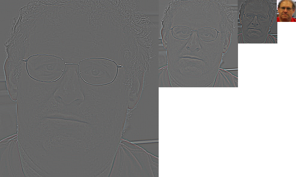
We can also verify whether we have constructed a valid Laplacian pyramid by collaplsing the pyramid into the original image. Collapsing a Laplacian pyramid is done by upsampling the last layer and adding it to the next layer in order to obtain a Gaussian pyramid. The following code verifies if the collapsing the Laplacian pyramid returns the identical image.


# reconstructing the original frame
_first_frame = (np.dot(yiq_video_gaussian_pyramid['g0'][0], yiq2rgb.T) * 255).astype(np.uint8)
_reconstructed_first_frame = cv2.pyrUp(
                                cv2.pyrUp(
                                    cv2.pyrUp(yiq_video_laplacian_pyramid['l3'][0]) \
                                        + yiq_video_laplacian_pyramid['l2'][0]) \
                                    + yiq_video_laplacian_pyramid['l1'][0]) \
                                + yiq_video_laplacian_pyramid['l0'][0]
_reconstructed_first_frame = (np.dot(_reconstructed_first_frame, yiq2rgb.T) * 255).astype(np.uint8)
cv2.imwrite('1_Reconstructed_Pyramid.png', cv2.cvtColor(_reconstructed_first_frame, cv2.COLOR_RGB2BGR))

print('Reconstructed images are '
    f'{"identical" if np.array_equal(_first_frame, _reconstructed_first_frame) else "different"}')

Temporal Filtering

Now for the main event, we will apply the same bandpass filter for each pixel along the temporal axis. For ideal filters, we convert the signal into the frequency domain using the np.fft module. Specifically, the rfft function does not return the redundant half of the Fourier transform result and enables us to directly mask certain frequencies to zero. A signle index of the DFT result corresponds to FPS/FRAME_COUNT Hz of the origianl signal. We return the signal after passing the bandpass filter so that we can amplify this signal by a specified constant AMP_VALUE. For butterworth filters, we use the scipy.signal library for both creating and applying filters to videos, which can be easily done with a few lines.


# create filter
if video_name == 'face':
    LOW_FREQ, HIGH_FREQ = 0.83, 1.0
    AMP_VALUE = 100
    sos = None
elif video_name == 'baby':
    LOW_FREQ, HIGH_FREQ = 0.4, 3
    AMP_VALUE = 10
    sos = signal.butter(1, [LOW_FREQ, HIGH_FREQ], btype='band', output='sos', fs=FPS)
elif video_name == 'baby2':
    LOW_FREQ, HIGH_FREQ = 2.33, 2.67
    AMP_VALUE = 150
    sos = None
elif video_name == 'subway':
    LOW_FREQ, HIGH_FREQ = 3.6, 6.2
    AMP_VALUE = 15
    sos = signal.butter(1, [LOW_FREQ, HIGH_FREQ], btype='band', output='sos', fs=FPS)
elif video_name == 'watch':
    LOW_FREQ, HIGH_FREQ = 4, 12
    AMP_VALUE = 10
    sos = signal.butter(1, [LOW_FREQ, HIGH_FREQ], btype='band', output='sos', fs=FPS)
else:
    raise NotImplementedError

# visualize filter
plt.figure(0)
if sos is not None:
    NYQ = 0.5 * FPS
    w, h = signal.sosfreqz(sos, worN=2048)
    plt.plot((NYQ / np.pi) * w, abs(h))
else:
    w = np.linspace(0, 15, 2048)
    h = [1 if LOW_FREQ <= x and x <= HIGH_FREQ else 0 for x in w]
    plt.plot(w, h)

def band_pass_filter(data, low_cut, high_cut, fs):
    low_cut, high_cut = int(low_cut * FRAME_COUNT / fs), int(high_cut * FRAME_COUNT / fs)
    rfft = np.fft.rfft(data, axis=0)
    rfft[:low_cut] = 0
    rfft[high_cut+1:] = 0
    return np.fft.irfft(rfft, n=FRAME_COUNT, axis=0).real

yiq_video_laplacian_pyramid_amplified = {}
for stage, video in sorted(yiq_video_laplacian_pyramid.items()):
    if sos is None:
        if stage in ['l0', 'l1']:
            yiq_video_laplacian_pyramid_amplified[stage] = yiq_video_laplacian_pyramid[stage]
            continue
        yiq_video_laplacian_pyramid_amplified[stage] = yiq_video_laplacian_pyramid[stage] \
                                    + band_pass_filter(yiq_video_laplacian_pyramid[stage], \
                                    LOW_FREQ, HIGH_FREQ, FPS) * AMP_VALUE
    else:
        yiq_video_laplacian_pyramid_amplified[stage] = yiq_video_laplacian_pyramid[stage] \
                                    + signal.sosfilt(sos, yiq_video_laplacian_pyramid[stage], axis=0)\
                                    * AMP_VALUE

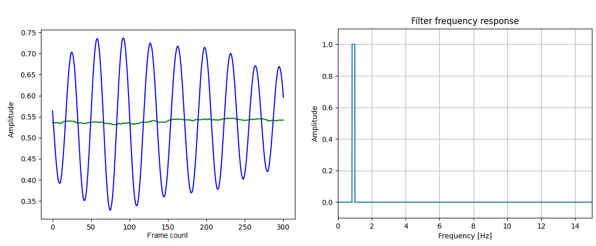
Bellow are the amplified signal and the bandpass filter used for the "face.mp4" video.

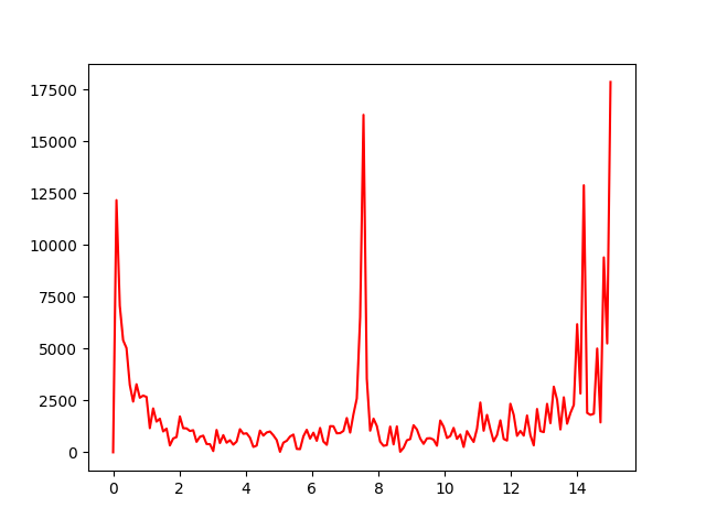
Extracting the Frequency Band of Interest

I was not successful at this problem, as I was not able to identify what frequencies should be amplified. For a naive start, I tried averaging along the spatial dimension to obtain a 1D-signal and analyzed the frequency of that signal. However, I was not able to find anything special near 1Hz. This seemed to be an obvious result since the frequency that needs to be amplified wouldn't have a high amplitude at the first place.


        yiq_video_averaged = np.sum(yiq_video, axis=(1,2,3))
        yiq_video_averaged_fft = np.fft.fft(yiq_video_averaged, axis=0)

        # Remove DC component
        yiq_video_averaged_fft[(FRAME_COUNT+1)//2] = 0.

        plt.figure(2)
        f = np.linspace(0, FPS//2, FRAME_COUNT//2)
        plt.plot(f, np.abs(yiq_video_averaged_fft)[(FRAME_COUNT + 1) // 2:], color='r')
        plt.savefig('3_Frequency_Analysis.png')

I think the best effort would be to use specific domain knowledge. (e.g., heartbeat is around 0.83Hz - 1.0Hz)

Image Reconstruction

Collapsing the Laplacian pyramid is the same process as seen above. The results for blood flow amplification are seen bellow. The video has some artifacts in regions out-of-interest since the original paper proposed extensive spatial filtering which our project did not consider.

We also experiment on the motion-magnification videos provided in the original paper, namely "baby.mp4" and "subway.mp4". We can observe the motions getting amplified even though we did not perform any spatial-aware operation.


print('Saving video...')

fourcc = cv2.VideoWriter_fourcc(*'mp4v')
writer = cv2.VideoWriter(f'5_Amplified_{video_name}.mp4', fourcc, FPS, (WIDTH, HEIGHT))

for i in range(FRAME_COUNT):
  yiq_reconstructed_frame = cv2.pyrUp(
                              cv2.pyrUp(
                                  cv2.pyrUp(yiq_video_laplacian_pyramid_amplified['l3'][i]) \
                                      + yiq_video_laplacian_pyramid_amplified['l2'][i]) \
                                  + yiq_video_laplacian_pyramid_amplified['l1'][i]) \
                              + yiq_video_laplacian_pyramid_amplified['l0'][i]

  _rgb_reconstructed_frame = np.clip(np.dot(yiq_reconstructed_frame, yiq2rgb.T), 0, 1)
  rgb_reconstructed_frame = (_rgb_reconstructed_frame * 255).astype(np.uint8)
  frame = cv2.cvtColor(rgb_reconstructed_frame, cv2.COLOR_RGB2BGR)
  writer.write(frame)

writer.release()

Capture and Motion-Magnify Your Own Video

I recorded the bunny inside my watch jump up and down with my smart phone. My aim was to magnify the bunny's motion, but I ended up finding some parameters that magnify the moire patterns, leading to the bunny being colorful.

I amplified the signals between 0.5Hz to 3Hz with the butterworth filter with a factor of 10.