We will be implementing a poisson image blending technique introduced in the paper
"Poisson Image Editing" (SIGGRAPH 2003).
The codes are written in Python >=3.8 with the help of some basic libraries.
In order to run the code, first unzip the codes and run
pip install -r requirements.txt
in the desired Python enviornment.
        import os

        from collections import defaultdict

        import numpy as np

        import cv2

        import scipy.sparse

        from scipy.sparse import linalg
We will first practice reconstructing an image given a single pixel value and the gradient values for all pixels. In order to do so, we need to formulate this problem as a least square problem, expressed as Ax = b. We will first express all the laplcian filter as a matrix A, which can be done with the following code. The size of matrix A is (H+2) × (W+2) to express padded values.
        toy_image = cv2.cvtColor(cv2.imread(f'data/toy_problem.png'), cv2.COLOR_BGR2GRAY)

        H, W = toy_image.shape


        # Laplacian filter on padded image

        A_1 = scipy.sparse.lil_matrix(((H+2)*(W+2), (H+2)*(W+2)))

        A_1.setdiag(-1, -1)

        A_1.setdiag(4)

        A_1.setdiag(-1, 1)

        A_1.setdiag(-1, 1*(W+2))

        A_1.setdiag(-1, -1*(W+2))
This condition is inaccurate at the boundary pixels, which are padded pixels, and thus we will not impose a laplacian objective on those pixels.
A_1[:W+2] = scipy.sparse.eye(W+2, (H+2)*(W+2), k=0)
A_1[-(W+2):] = scipy.sparse.eye(W+2, (H+2)*(W+2), k=(H+2)*(W+2) - (W+2))

for i in range(1,H+1):
    _temp = scipy.sparse.lil_matrix((1,(H+2)*(W+2)))
    _temp[0, i*(W+2)] = 1
    A_1[i*(W+2)] = _temp.copy()
    _temp = scipy.sparse.lil_matrix((1,(H+2)*(W+2)))
    _temp[0, i*(W+2) + (W+1)] = 1
    A_1[(i*(W+2) + (W+1))] = _temp.copy()
Now we will add a row to indicate the value of the single point at (0, 0).
        A_2 = scipy.sparse.lil_matrix((1,(H+2)*(W+2)))

        A_2[0,(W+2)]= 1

        A = scipy.sparse.vstack([A_1, A_2])
We will consturct the vecotr b with the corresponding laplacian values and the padded values.
This can be easily done with the cv2.filter2D method.
            kernel = np.array([[ 0,-1, 0], [-1, 4,-1], [ 0,-1, 0],], dtype=np.float32)

            _padded_image = cv2.copyMakeBorder(toy_image, 1, 1, 1, 1, cv2.BORDER_DEFAULT).astype(np.float32)

            b = cv2.filter2D(toy_image, cv2.CV_32F, kernel)

            _padded_image[1:-1, 1:-1] = b.copy()

            b = np.reshape(_padded_image, ((H+2)*(W+2), 1))

            b = np.append(b, [toy_image[0,0]])
All that is left for us to do is solve the least square problem Ax=b.
The scipy.sparse.linalg.lsqr provides a solution given sparse matrices with minimum computational cost.
This gives us the reconstructed images.
            x = linalg.lsqr(A, b, atol=1e-10, btol=1e-10)[0]

            new_image = x.reshape(H+2,W+2)

            new_image = new_image[1:-1, 1:-1]


            new_image = np.clip(new_image, 0, 255).astype(np.uint8)

            cv2.imwrite('1_toy_problem.png', new_image)
 -->
-->
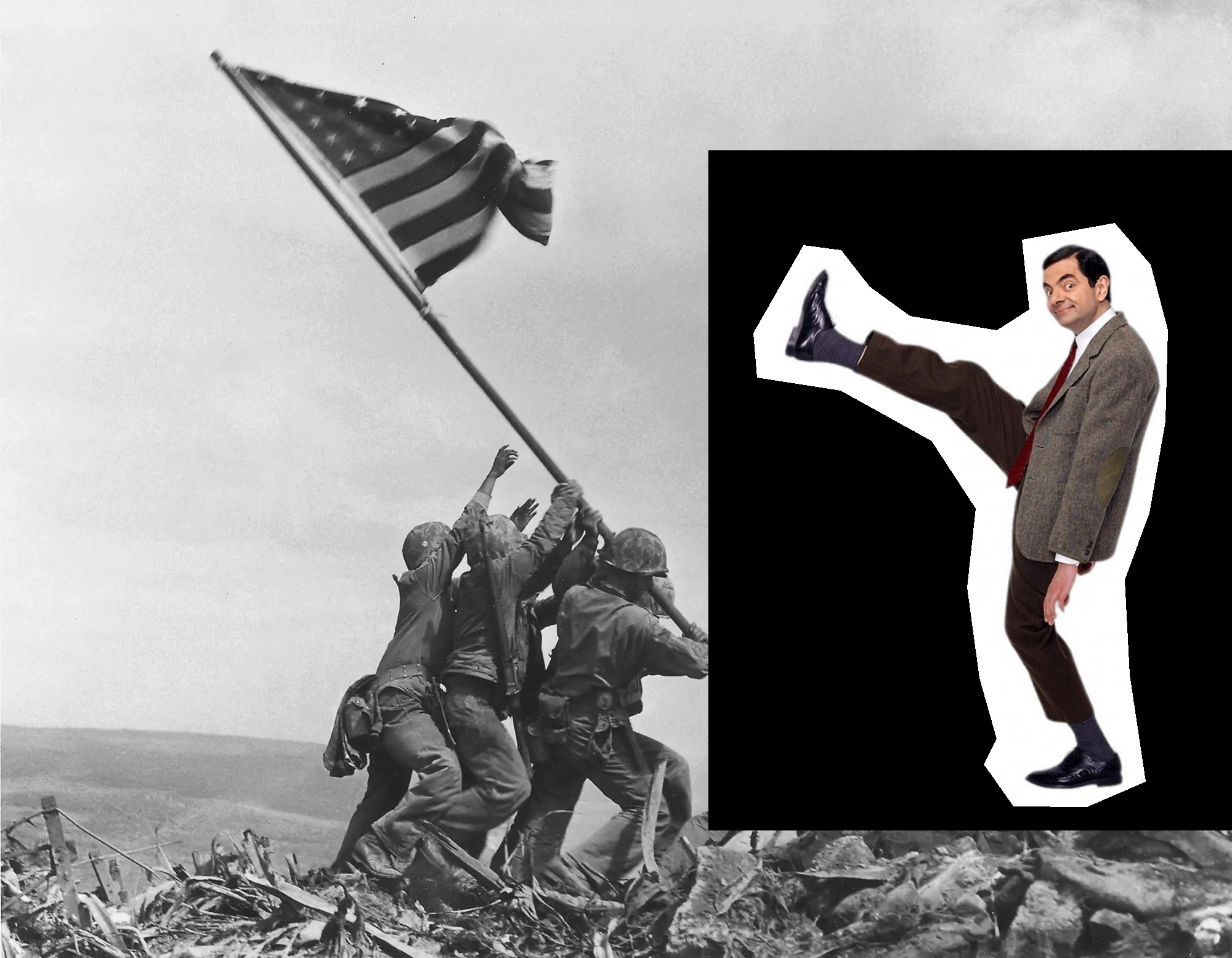
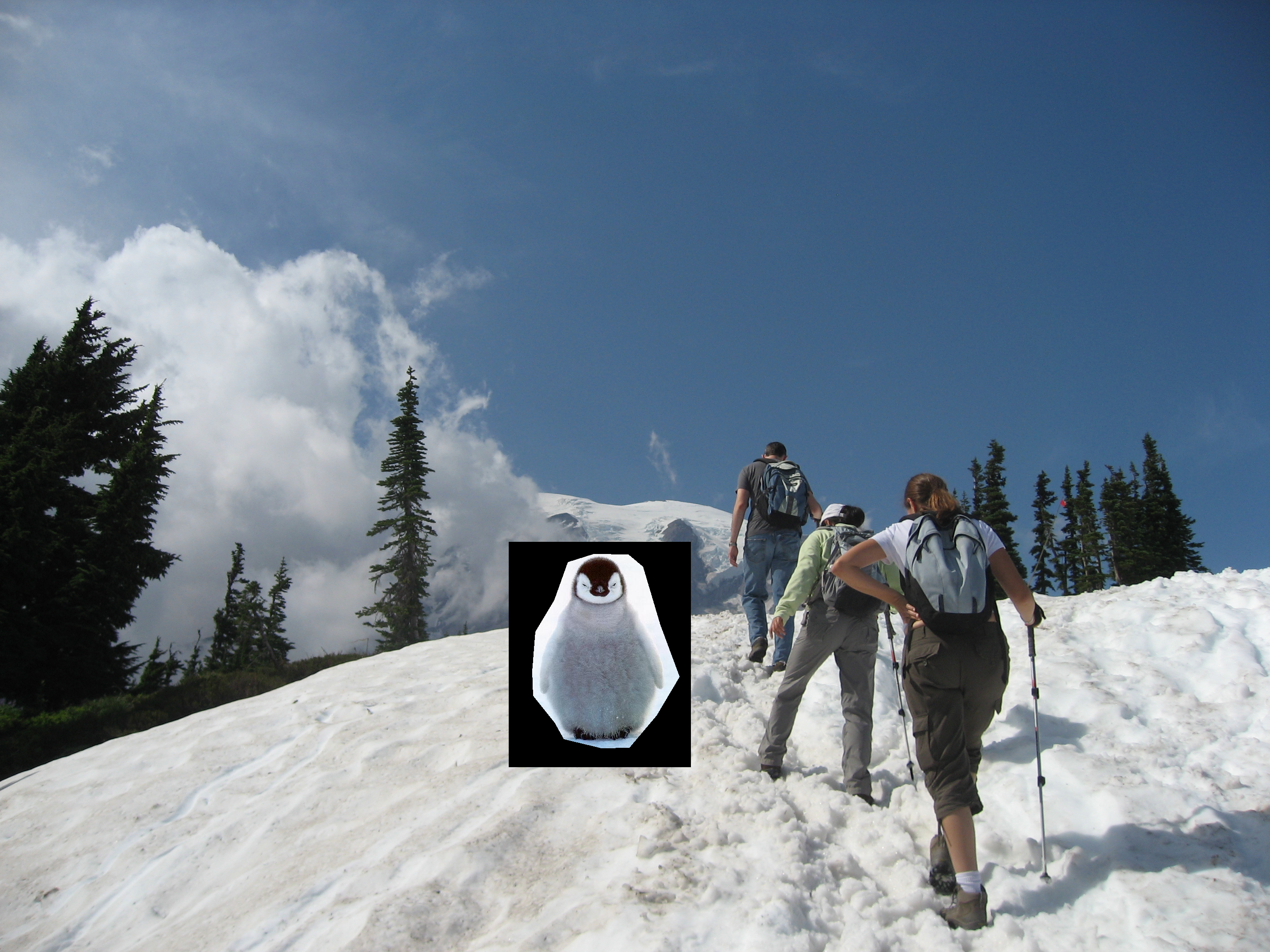
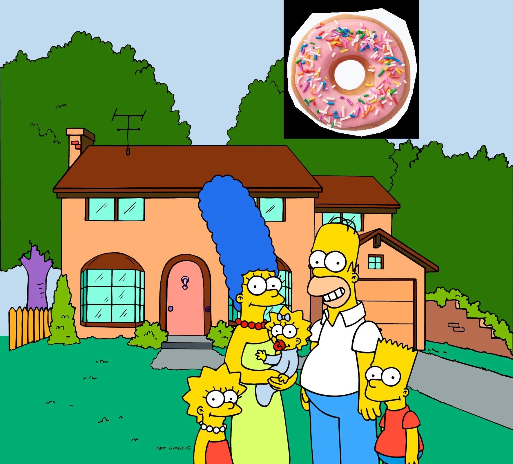
We will implement poisson blending in a similar manner, but now we only consider the pixels in the source image region rather than the entire image. Before constructing the matrices A and b, the following code shows how the source and target images are preprocessed. Specifically, I created a mask selection tool and a mask pasting tool to allow the user to select the region of interest. For the full details of the tools, please refer to the source codes.
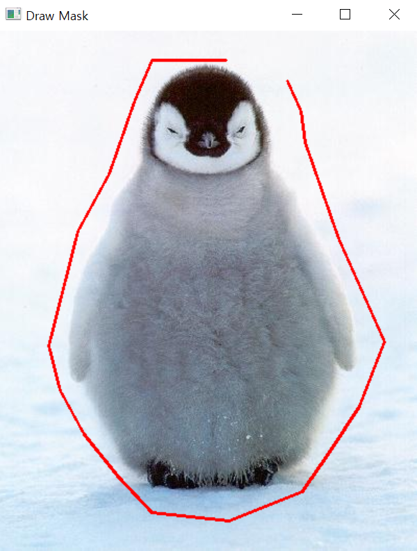

Given a mask of the source image and the desired location in the target image, we first resize the
Then we obtain the boundary region using the cv2.findContours function and subtract the regions that overlap with the mask.
In this way, we can identify the source image region and the neighboring pixels.
# Read source image
src_image = cv2.imread(f'data/{SRC_IMAGE}.jpg') # XXX
SRC_H, SRC_W = src_image.shape[0], src_image.shape[1]
src_image = cv2.resize(src_image, ((SRC_W//2) * 2, (SRC_H//2) * 2))
SRC_H, SRC_W = src_image.shape[0], src_image.shape[1]
# Select mask from the source image
if os.path.exists(f'./data/{SRC_IMAGE}-mask.png'):
src_masked = cv2.imread(f'./data/{SRC_IMAGE}-masked.png')
src_mask = cv2.imread(f'./data/{SRC_IMAGE}-mask.png')
else:
mask_gui = MaskSelectionTool(src_image)
src_masked, src_mask = mask_gui.draw()
cv2.imwrite(f'./data/{SRC_IMAGE}-masked.png', src_masked)
cv2.imwrite(f'./data/{SRC_IMAGE}-mask.png', src_mask)
src_mask = src_mask[:,:,0]
# Read target image
tgt_image = cv2.imread(f'data/{TGT_IMAGE}.jpg') # XXX
TGT_H, TGT_W, TGT_C = tgt_image.shape[0], tgt_image.shape[1], tgt_image.shape[2]
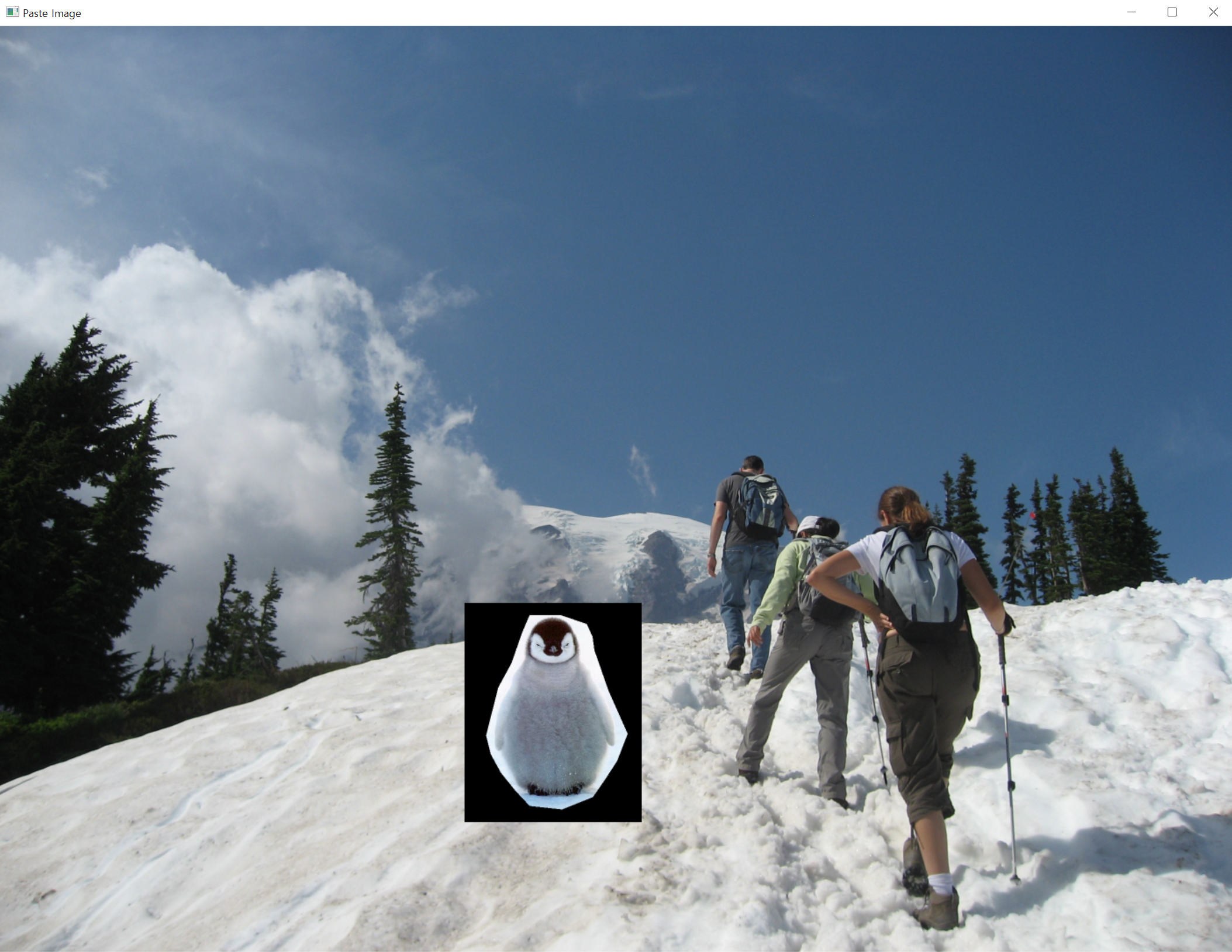
# Select where to paste the mask
paste_gui = MaskInjectionTool(tgt_image, src_masked, resize_ratio=2)
(click_w, click_h), canvas = paste_gui.draw()
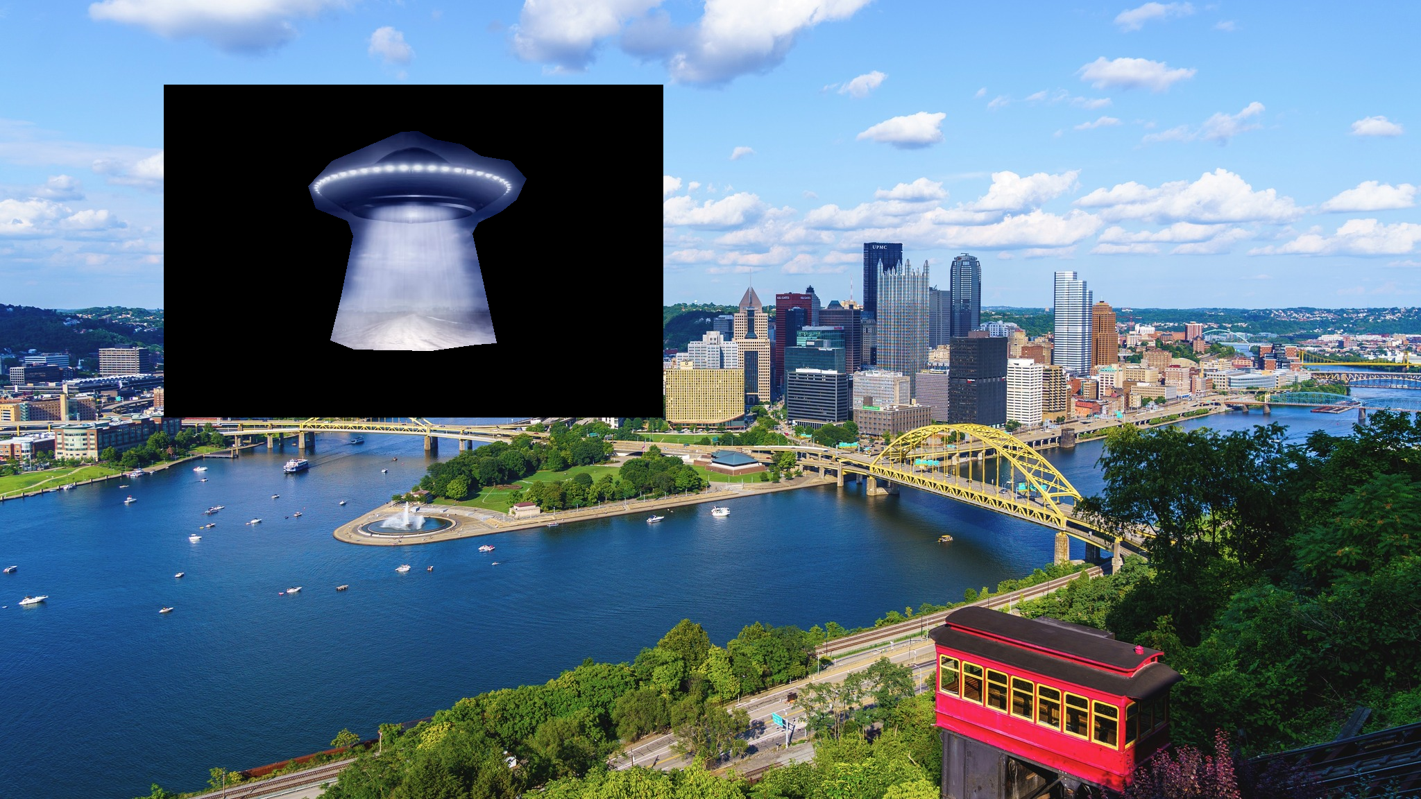
cv2.imwrite('2_before_blending.png', canvas)
src_image_padded = np.zeros_like(tgt_image)
src_image_padded[click_h - SRC_H//2: click_h + SRC_H//2,
click_w - SRC_W//2: click_w + SRC_W//2] = src_image
kernel = np.array([[ 0,-1, 0],
[-1, 4,-1],
[ 0,-1, 0],], dtype=np.float32)
src_gradient = cv2.filter2D(src_image_padded, cv2.CV_32F, kernel)
src_mask_padded = np.zeros((TGT_H, TGT_W), dtype=np.uint8)
src_mask_padded[click_h - SRC_H//2: click_h + SRC_H//2,
click_w - SRC_W//2: click_w + SRC_W//2] = src_mask
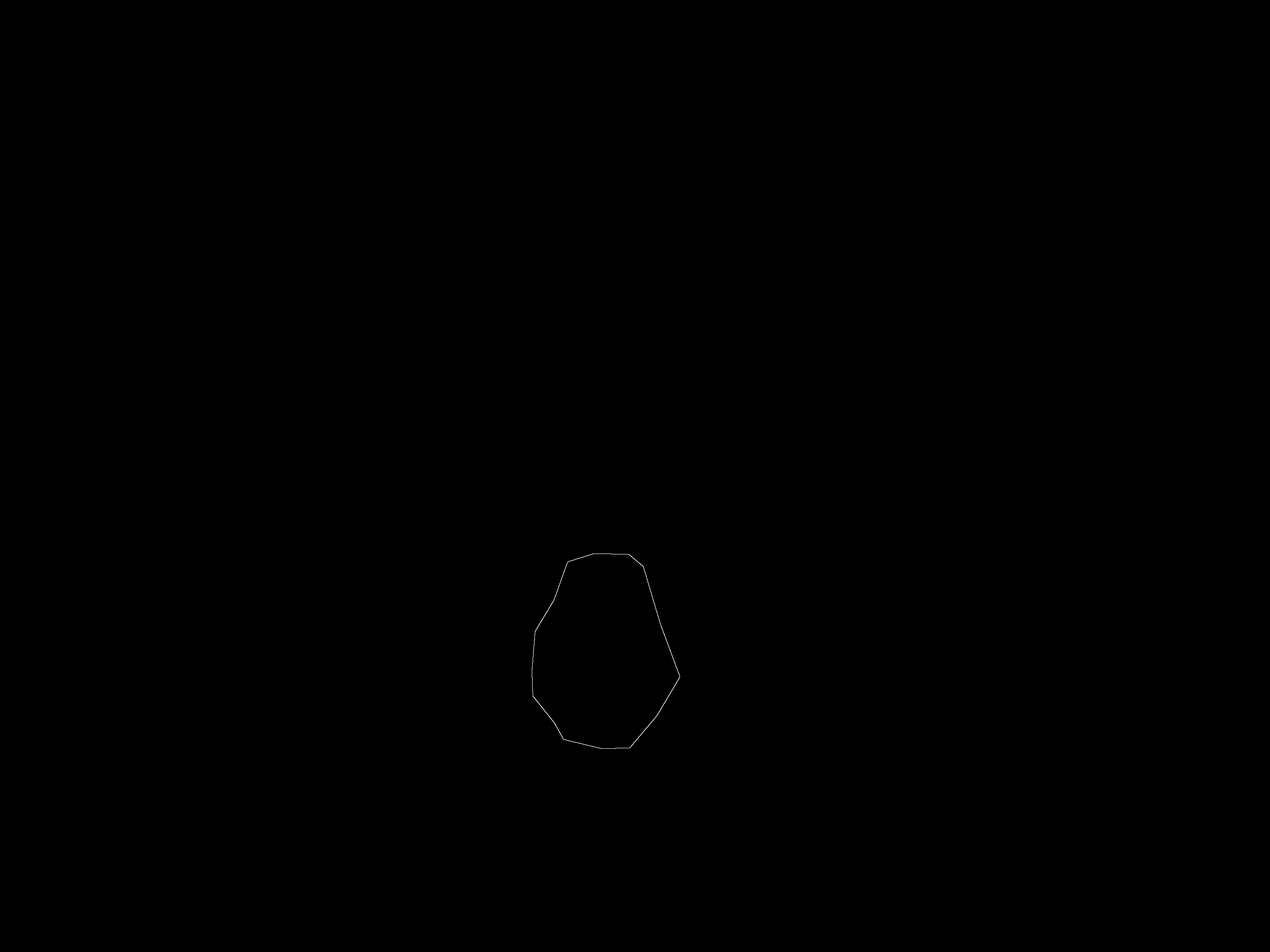
# Omega delta region index
_contour, _hierarchy = cv2.findContours(src_mask_padded, cv2.RETR_EXTERNAL, cv2.CHAIN_APPROX_NONE)
_omega_delta_map = cv2.drawContours(np.zeros_like(src_mask_padded), _contour, -1, 255, 2, cv2.LINE_4, _hierarchy)
_omega_delta_map = cv2.subtract(_omega_delta_map, src_mask_padded)
omega_delta_indices = np.nonzero(_omega_delta_map)
omega_delta_indices = [(x, y) for x,y in zip(omega_delta_indices[0], omega_delta_indices[1])]
cv2.imwrite('2_omega_delta_region.png', _omega_delta_map)
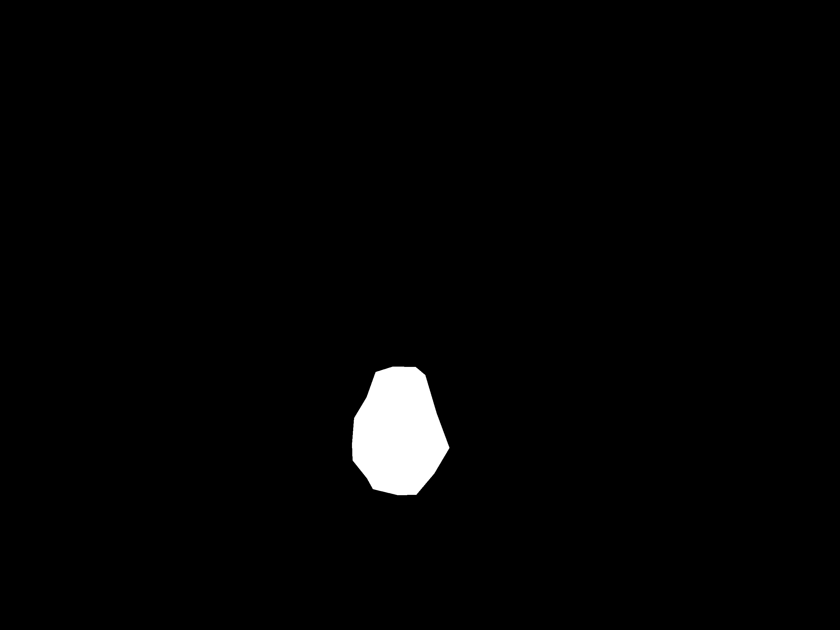
# Omega region index
omega_indices = np.nonzero(src_mask_padded)
omega_indices = [(x, y) for x,y in zip(omega_indices[0], omega_indices[1])]
cv2.imwrite('2_omega_region.png', src_mask_padded)
index2point and point2index.
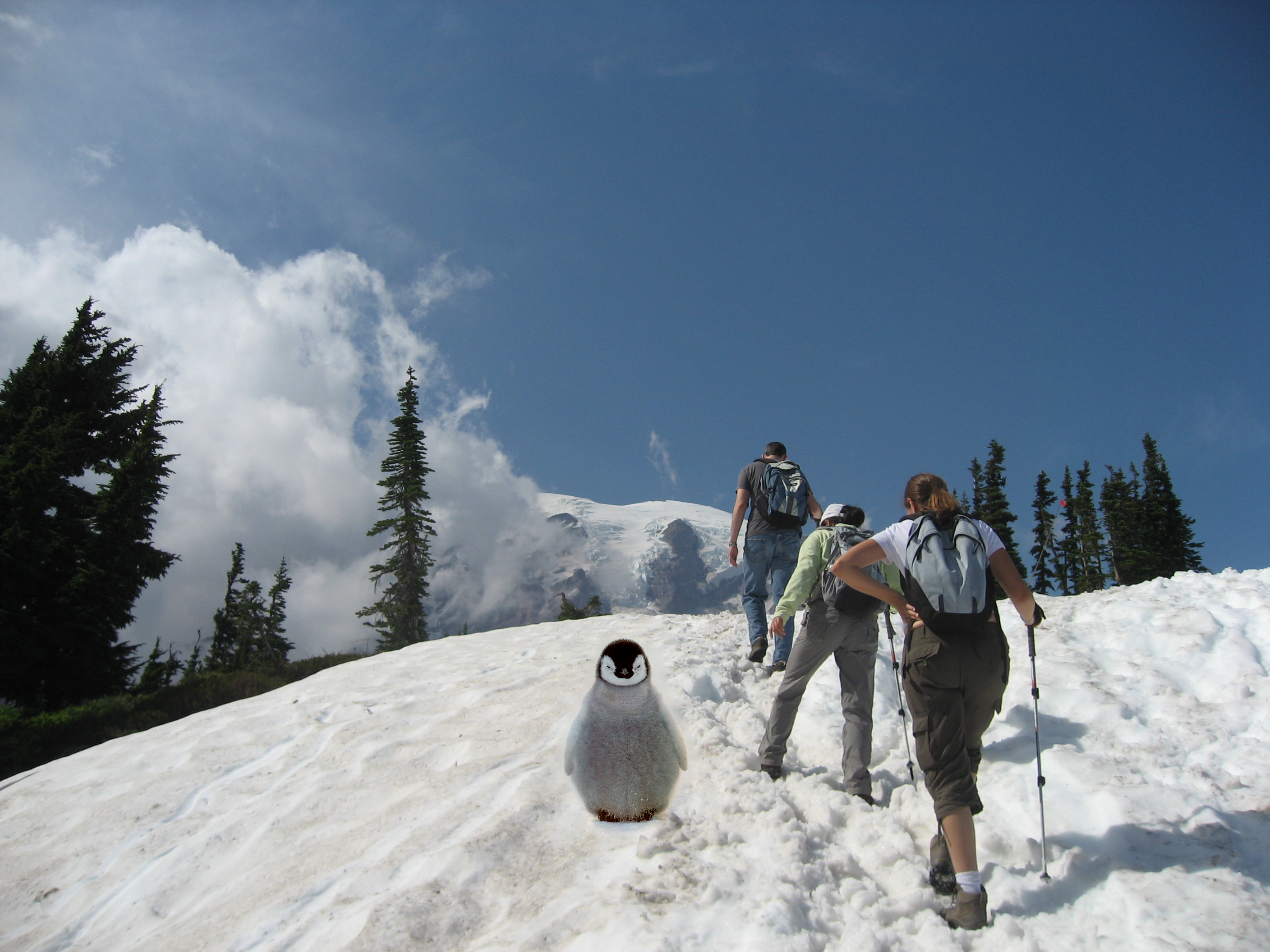
We construct the matrices A and b utilizing these two dictionaries and solve for x.
we paste the new source image onto the target image to finish our poisson blending procedure.
N = len(omega_delta_indices) + len(omega_indices)
A = scipy.sparse.lil_matrix((N, N))
b = np.zeros(N)
index2point = defaultdict(tuple)
point2index = {}
for i, point in enumerate(omega_indices + omega_delta_indices):
index2point[i] = point
point2index[point] = i
print('Solving matrix...')
blended = np.zeros((len(omega_indices), TGT_C))
for ch in range(TGT_C):
for point in omega_delta_indices:
h, w = point[0], point[1]
i = point2index[point]
A[i, i] = 1
b[i] = tgt_image[h, w, ch]
for point in omega_indices:
h, w = point[0], point[1]
i = point2index[point]
A[i, i] = 4
neighbor = [(h, w+1), (h+1, w), (h-1, w), (h, w-1)]
neighbor_idx = [point2index[p] for p in neighbor]
A[i, neighbor_idx] = -1
b[i] = src_gradient[h,w, ch]
x = linalg.spsolve(A.tocsc(), b)
x = np.clip(x[:len(omega_indices)], 0, 255)
blended[:,ch] = x
# insert to target image
print('Blending the two images...')
blended_image = tgt_image.copy()
for i, value in enumerate(blended):
h, w = index2point[i]
blended_image[h, w] = value
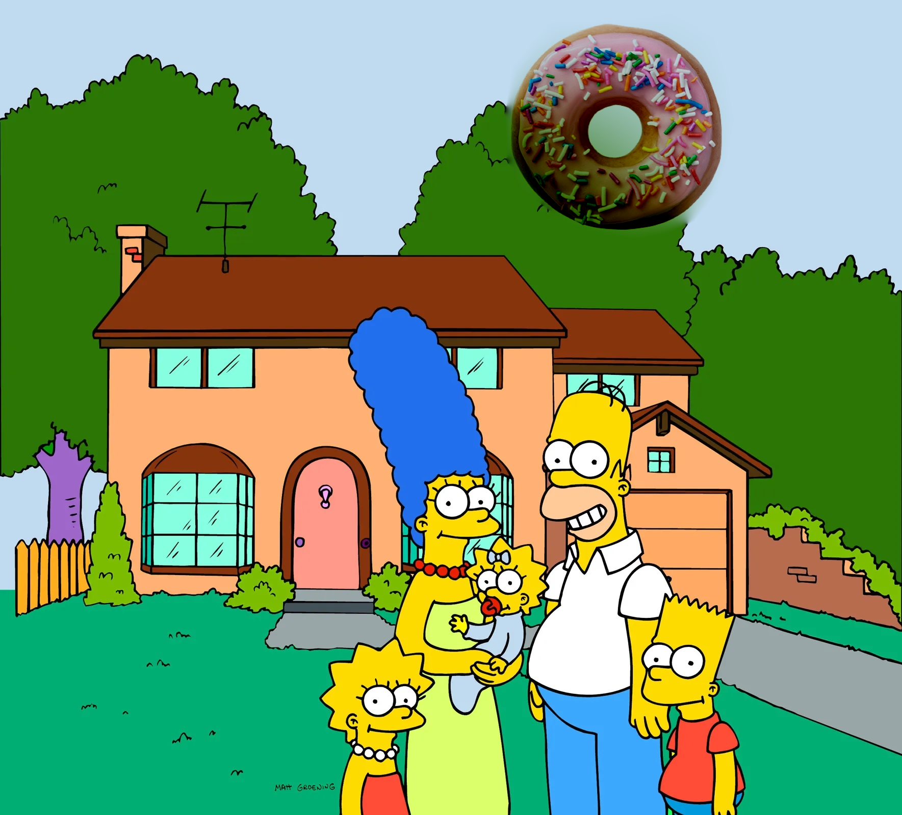
cv2.imwrite('2_poisson_blending.png', blended_image)
The origianl paper also suggests using mixed gradients, which utilizes target image gradients when they are larger than the source image gradients. We can fill in holes that are flat in the source image with the gradient of the target image. We simply change the src_gradient to a mix_gradient with the following code.
print('Mixing gradients...')
tgt_gradient = cv2.filter2D(tgt_image, cv2.CV_32F, kernel)
mix_gradient = np.zeros_like(tgt_gradient)
src_is_larger = np.abs(src_gradient) > np.abs(tgt_gradient)
mix_gradient = src_is_larger * src_gradient + ~src_is_larger * tgt_gradient
A = scipy.sparse.lil_matrix((N, N))
b = np.zeros(N)
# Reuse A matrix
print('Solving matrix...')
mix_blended = np.zeros((len(omega_indices), TGT_C))
for ch in range(TGT_C):
for point in omega_delta_indices:
h, w = point[0], point[1]
i = point2index[point]
A[i,i] = 1
b[i] = tgt_image[h, w, ch]
for point in omega_indices:
h, w = point[0], point[1]
i = point2index[point]
A[i, i] = 4
neighbor = [(h, w+1), (h+1, w), (h-1, w), (h, w-1)]
neighbor_idx = [point2index[p] for p in neighbor]
A[i, neighbor_idx] = -1
b[i] = mix_gradient[h,w, ch]
x = linalg.spsolve(A.tocsc(), b)
# breakpoint()
x = np.clip(x[:len(omega_indices)], 0, 255)
mix_blended[:,ch] = x
# insert to target image
mix_blended_image = tgt_image.copy()
for i, value in enumerate(mix_blended):
h, w = index2point[i]
mix_blended_image[h, w] = value
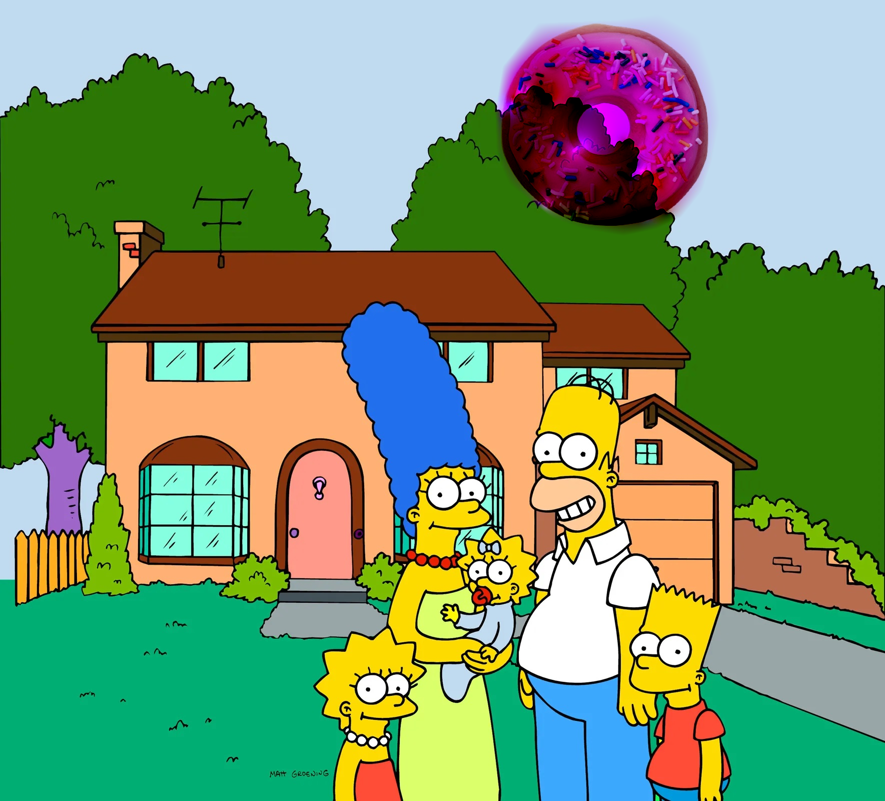
cv2.imwrite('3_mixed_blending.png', mix_blended_image)
The effect of mixed gradients can be seen in the example bellow. The doughnut hole is filled in with the background of the target image. However, some colors are lost by giving an imperfect gradient guidance.
To assess the poisson blending and mixed gradient blending approaches, we provide three cases for comparison.
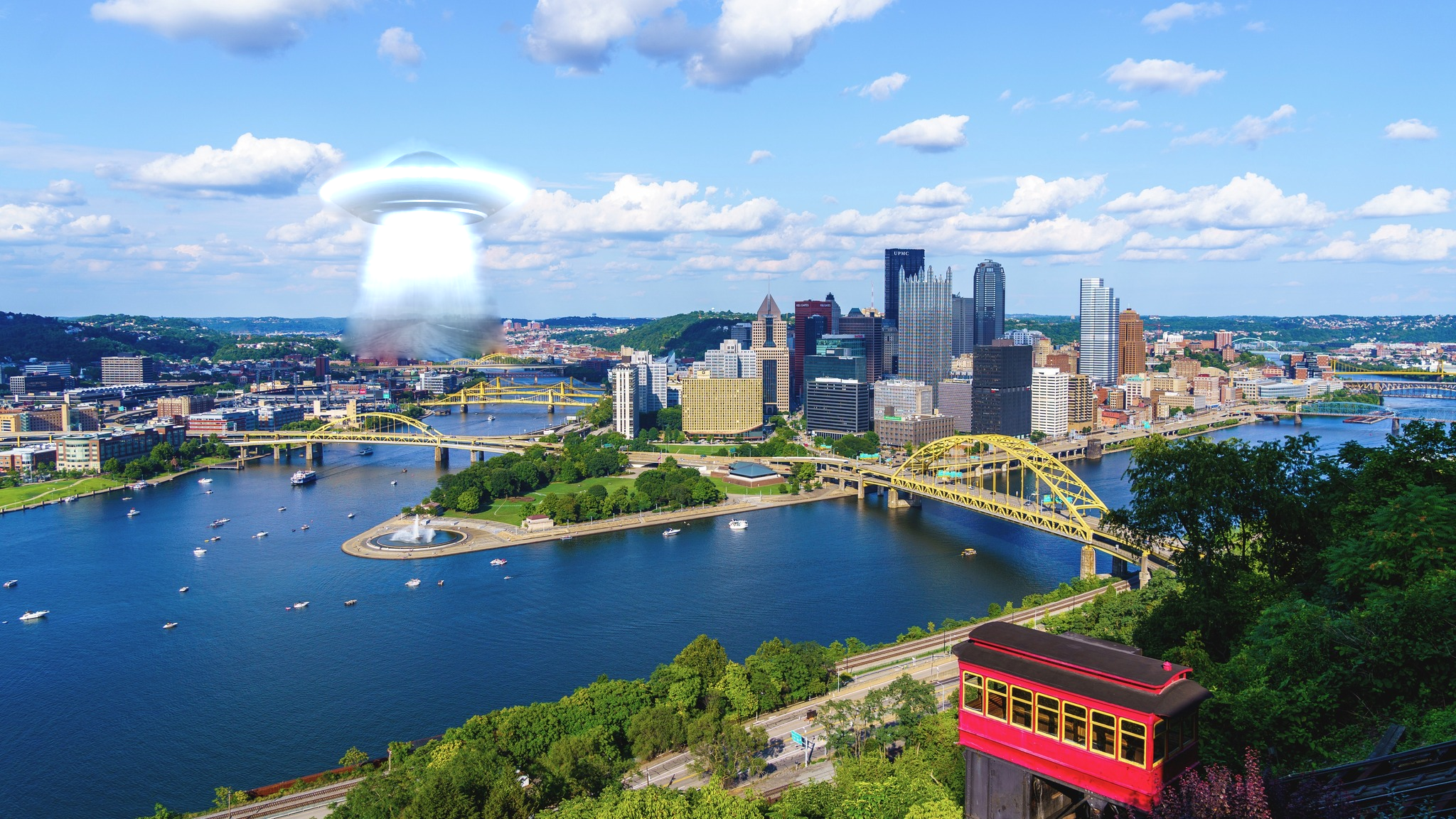
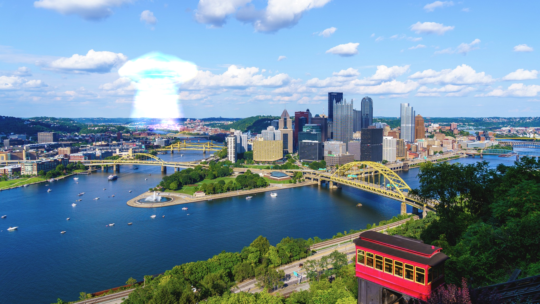
The first example is a blending example of a UFO over a city skyline. Notice that the source image (UFO) is from a dark background with low contrast. Thus, the UFO is bright and hard to detect, just like how you would see one in daylight. However, the dirt road under the UFO beam covers the original background. Using mixed gradient resolves this issue and properly shows the city under the beam of light. However, the UFO becomes even more fainter as it looses texture.
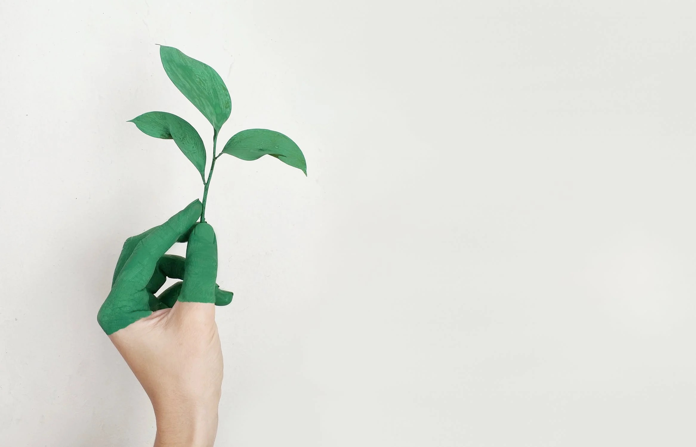
Another good example of poisson blending can be seen in the next example. Poisson blending is often prone to changing colors in the background as seen in the second image. Also, the doughnut ring is filled with the contents from the source and blocks the tree behind. When using mixed gradients, the tree behind the doughnut is visible. However, we can notice that too much of it is visible, making the doughnut transparent.
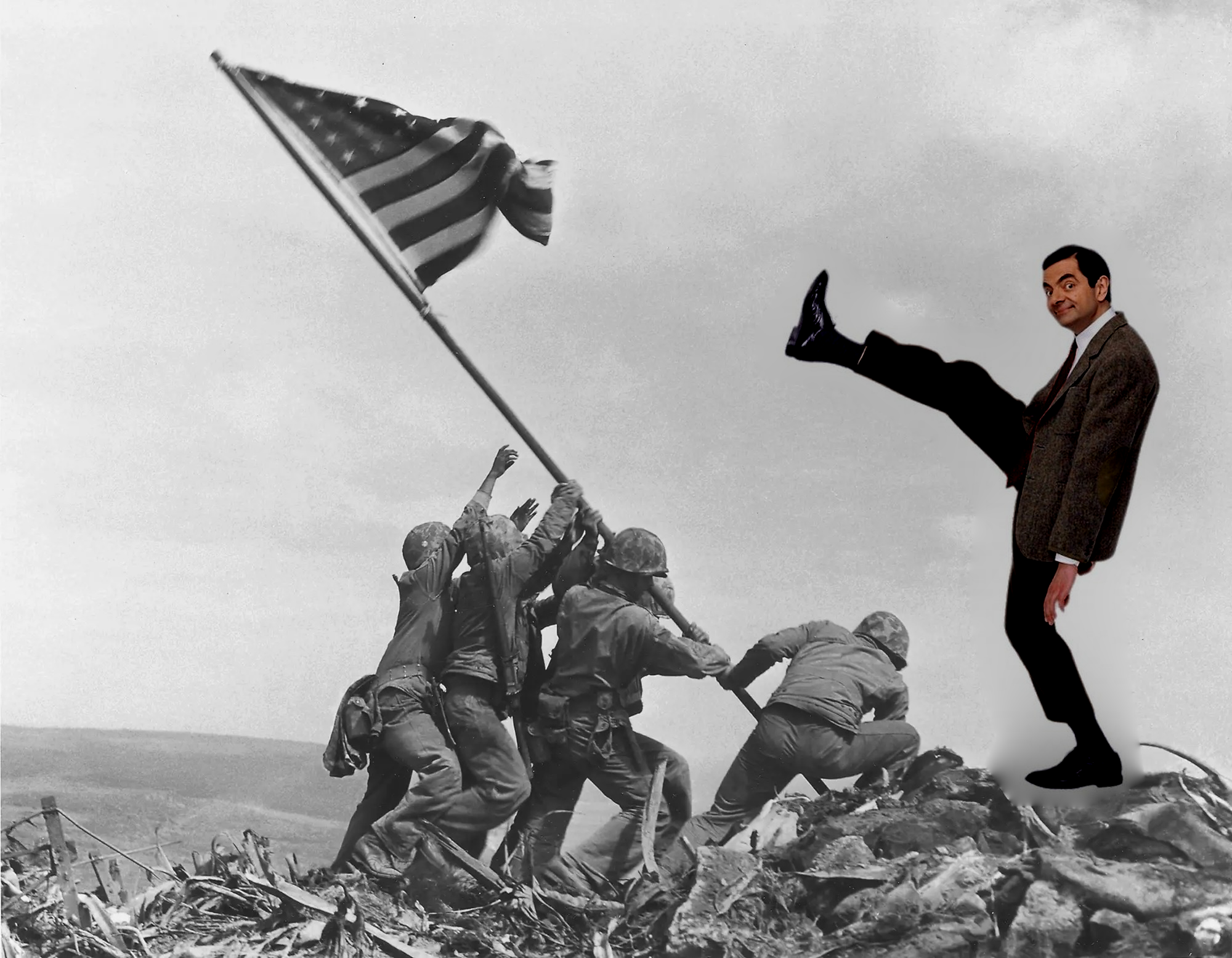
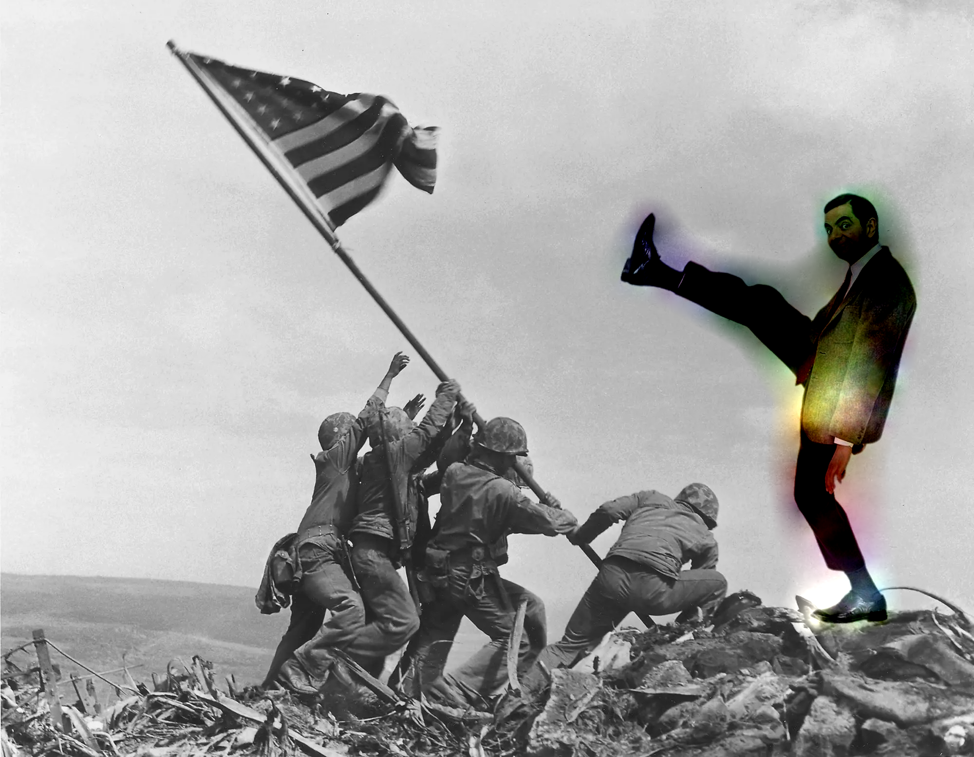
Another failure case of using mixed gradients. When using normal poisson blending, Mr.Bean is seamlessly pasted onto the historic photo. However, when using mixed gradients, the brightness of the source image becomes inconsistent. This is due to the small but relevant gradients in the target image, which tends to get amplified when taken the max gradients.